// Code and ☕ with Mason

Home

CUDA Kernel Grid, Block, and Thread Structure

Published: Feb 8th, 2024

Apple Silicon Assembly Code

NVIDIA's CUDA technology introduces a hierarchy of thread organization that is pivotal in exploiting the parallel processing capabilities of the NVIDIA hardware. This article aims to clarify how CUDA kernel invocations shape the grid and blocks structure and how developers can control thread configurations within blocks using the 'blockDim' variable.

Kernel Invocations and Grid Structure

When a CUDA kernel is invoked, it spawns a new execution grid composed of multiple thread blocks. The grid serves as the top-level structure for organizing threads in a way that reflects the GPU's capability to execute many threads in parallel. Each block within the grid can house up to 1024 individual threads—although this maximum limit is subject to change with newer generations of GPUs and can be verified by consulting the latest CUDA Programming Guide.

Block Composition and Shared Memory

Threads within the same block have the unique advantage of being able to communicate through a shared memory region colloquially known as SMEM. This low-latency memory space is exclusive to the block, allowing threads to exchange data rapidly without resorting to slower global memory transactions. Access to shared memory is synchronized, ensuring that data integrity is maintained throughout the block's execution lifetime.

Configuring Threads per Block with 'blockDim'

The configuration of threads within a block is flexible and can be tailored to the demands of specific applications. This is achieved using the 'blockDim' variable, which is a three-component vector of type 'int'. It defines the dimensionality (x, y, z) of each block within the grid. By adjusting these values, developers can optimize performance based on factors such as memory constraints and the nature of the algorithm being implemented.


    // Example of a kernel invocation with block dimension configuration
    __global__ void myKernel() {
        // Kernel code here
    }
    
    int main() {
        dim3 blockDim(16, 16, 1); // Configure a block of 256 threads (16x16)
        int numBlocks = ...;       // Determine the number of blocks required
        myKernel<<>>(); // Invoke the kernel
        cudaDeviceSynchronize();   // Synchronize the device
        return 0;
    }
            

To summarize, the CUDA programming model provides a hierarchical and efficient thread organization that is paramount for achieving parallelism on a GPU. Through careful configuration of grid and block dimensions, notably via the 'blockDim' variable, CUDA programmers have precise control over the execution of their kernels, enabling them to harness the compute power of GPUs for a variety of complex computational tasks.

Exploring CUDA Parallelism

Published: Feb 7th, 2024

CUDA (Compute Unified Device Architecture) is a parallel computing platform and programming model invented by NVIDIA. It enables dramatic increases in computing performance by harnessing the power of the graphics processing unit (GPU). In this article, we delve into the central features of CUDA architecture, such as streaming multiprocessors, registers, shared memory, and load/store units, and discuss how they contribute to achieving highly parallelized computation, especially in mathematical operations like matrix multiplication.

Streaming Multiprocessors (SMs)

The streaming multiprocessors are the heart of the CUDA-enabled GPU's ability to handle parallel tasks. Each SM can execute hundreds of threads concurrently, allowing for efficient division of workloads across a vast array of cores. This intrinsic parallelism makes GPUs exceptionally well-suited for algorithms that can be executed in parallel segments, such as the mathematically intensive operations found in linear algebra and deep learning.

Registers and Shared Memory

Each thread running on a CUDA GPU has access to its own private registers, providing fast access to variables. Meanwhile, shared memory allows for threads within the same block to communicate and share data quickly, reducing the need to access slower global memory and thus enhancing overall performance. Efficient use of both registers and shared memory is key to optimizing CUDA applications.

Load/Store Units

Load/store units are responsible for reading from and writing to memory. By efficiently managing these operations, CUDA minimizes memory bottlenecks. The architecture provides separate paths for loading data from global memory into registers and for storing results back from registers into memory, effectively overlapping memory operations with computation, which is crucial for maintaining high throughput.

Optimized Math Operations

CUDA's design is optimized for compute-intensive tasks. For example, matrix multiplication (matmul), a staple operation in many scientific and engineering computations, benefits greatly from CUDA's parallel execution capabilities. The abundant computational resources and the ability to perform many operations simultaneously lead to significant accelerations of matrix-matrix or matrix-vector products, which can be observed in the widespread use of CUDA in high-performance computing applications.

The combination of streaming multiprocessors, efficient memory hierarchy, and optimized data pathways enables CUDA to excel at parallel computation. Developers leveraging CUDA can achieve speedups that are orders of magnitude greater than those possible on traditional CPUs for certain tasks, making it an indispensable tool for modern computationally demanding applications.

Understanding Linearization of Abstract Syntax Trees

Published: Feb 7th, 2024

Linearization of Abstract Syntax Trees (ASTs) plays a crucial role in the compilation and interpretation of programming languages. It transforms the nested, hierarchical structure of an AST into a flat sequence of instructions, making it easier to perform optimizations and generate machine code. This article delves into the linearization process, using a specific example of an AST that represents a simple arithmetic operation and how it can be linearized into a sequence of operations suitable for further processing or execution.

The provided AST illustrates a lazy evaluation operation where two constants are added together, and the result is stored. The AST is structured to capture the computation of adding 2.0 and 3.0, followed by storing the result. This tree structure is rich in information but not in a format that's directly executable by a machine.


  LazyOp(
      op=BufferOps.STORE,
      src=(
          LazyOp(
              op=BinaryOps.ADD,
              src=(
                  LazyOp(
                      op=BufferOps.CONST,
                      src=(),
                      arg=ConstBuffer(
                          val=2.0,
                          dtype=dtypes.float,
                          st=ShapeTracker(
                              views=(
                                  View(
                                      shape=(),
                                      strides=(),
                                      offset=0,
                                      mask=None,
                                      contiguous=True
                                  ),
                              )
                          )
                      )
                  ),
                  LazyOp(
                      op=BufferOps.CONST,
                      src=(),
                      arg=ConstBuffer(
                          val=3.0,
                          dtype=dtypes.float,
                          st=ShapeTracker(
                              views=(
                                  View(
                                      shape=(),
                                      strides=(),
                                      offset=0,
                                      mask=None,
                                      contiguous=True
                                  ),
                              )
                          )
                      )
                  )
              ),
              arg=None
          ),
      ),
      arg=MemBuffer(
          idx=0,
          dtype=dtypes.float,
          st=ShapeTracker(
              views=(
                  View(
                      shape=(),
                      strides=(),
                      offset=0,
                      mask=None,
                      contiguous=True
                  ),
              )
          )
      )
  )
          

The linearization process translates this AST into a series of sequential operations, as shown below:

              
  UOps.DEFINE_GLOBAL  : ptr.dtypes.float          []                               data0
  UOps.CONST          : dtypes.float              []                               2.0
  UOps.CONST          : dtypes.float              []                               3.0
  UOps.ALU            : dtypes.float              [<UOps.CONST: 10>, <UOps.CONST: 10>] BinaryOps.ADD
  UOps.CONST          : dtypes.int                []                               0
  UOps.STORE          :                           [<UOps.DEFINE_GLOBAL: 5>, <UOps.CONST: 10>, <UOps.ALU: 13>] None


This linearized sequence starts with defining a global memory buffer for storing the result, followed by loading the constants 2.0 and 3.0. An arithmetic logic unit (ALU) operation then adds these constants. Finally, the result is stored in the previously defined global memory location. Each step is represented as an operation with specific operands and operation types, illustrating the direct and sequential nature of execution that linearization facilitates.

The transformation from a hierarchical AST to a linear sequence of operations enables the efficient execution of code by providing a clear path for compilers and interpreters. This example underscores the importance of linearizers in the optimization and execution phases of code compilation, showcasing their role in simplifying complex structures into actionable sequences.

Abstract Syntax Trees (ASTs)

Published: Feb 6th, 2024

Abstract Syntax Trees (ASTs) are hierarchical data structures used to represent the syntactic structure of code in programming languages. ASTs capture the structure of code independently of its textual representation, enabling developers to analyze and manipulate code programmatically. These trees are fundamental components of compilers, interpreters, and static analysis tools, facilitating tasks such as code optimization, transformation, and error detection.

Constructing an AST involves parsing source code and creating a tree structure that reflects its syntax. Each node in the tree corresponds to a syntactic element of the code, such as expressions, statements, or declarations. Traversing the AST allows for various analyses and transformations, making it a powerful tool.


    result = Tensor(2.0) + Tensor(3.0)       
          

The AST for the above code looks like:


    LazyOp(
      op=BufferOps.STORE,
      src=(
          LazyOp(
              op=BinaryOps.ADD,
              src=(
                  LazyOp(
                      op=BufferOps.CONST,
                      src=(),
                      arg=ConstBuffer(
                          val=2.0,
                          dtype=dtypes.float,
                          st=ShapeTracker(
                              views=(
                                  View(
                                      shape=(),
                                      strides=(),
                                      offset=0,
                                      mask=None,
                                      contiguous=True
                                  ),
                              )
                          )
                      )
                  ),
                  LazyOp(
                      op=BufferOps.CONST,
                      src=(),
                      arg=ConstBuffer(
                          val=3.0,
                          dtype=dtypes.float,
                          st=ShapeTracker(
                              views=(
                                  View(
                                      shape=(),
                                      strides=(),
                                      offset=0,
                                      mask=None,
                                      contiguous=True
                                  ),
                              )
                          )
                      )
                  )
              ),
              arg=None
          ),
      ),
      arg=MemBuffer(
          idx=0,
          dtype=dtypes.float,
          st=ShapeTracker(
              views=(
                  View(
                      shape=(),
                      strides=(),
                      offset=0,
                      mask=None,
                      contiguous=True
                  ),
              )
          )
      )
    )


And the generated clang code:


    void E_n2(float* restrict data0) {
      data0[0] = (2.0f+3.0f);
    }


This hierarchical structure captures the syntactic composition of the mathematical expression, enabling further analysis and manipulation of the code.

Interpreted vs. Compiled Backends

Published: Feb 5th, 2024

When it comes to executing code, software systems typically employ one of two approaches: interpreted or compiled backends. Understanding the differences between these approaches is crucial for developers, as they can significantly impact the performance and behavior of programs. In this post, we'll explore the distinctions between interpreted and compiled backends, along with a code example demonstrating each.

Interpreted Backend

In an interpreted backend, code is executed line by line or statement by statement by an interpreter at runtime. This means that the source code is translated into machine code or an intermediate representation just before execution. Interpreted languages offer flexibility and dynamism, but they may run slower than compiled code due to the overhead of interpretation.


    # Python Example: Interpreted Backend
    def add(a, b):
        return a + b
    
    result = add(5, 3)
    print(result)  # Output: 8
            

Compiled Backend

In contrast, a compiled backend translates the source code into machine code or bytecode ahead of time, typically during a separate compilation phase. This pre-compiled code can then be executed directly by the hardware or a virtual machine without further translation at runtime. Compiled code tends to run faster than interpreted code due to the elimination of runtime interpretation overhead.


    // C Example: Compiled Backend
    #include <stdio.h>
    
    int add(int a, int b) {
        return a + b;
    }
    
    int main() {
        int result = add(5, 3);
        printf("%d\n", result); // Output: 8
        return 0;
    }
            

As demonstrated in the code examples above, the choice between interpreted and compiled backends depends on various factors, including performance requirements, platform compatibility, and development preferences. Both approaches have their strengths and weaknesses, and understanding when to use each is essential for building efficient and effective software systems.

Neural Networks: Most Widely Used Optimizers

Published: Feb 4th, 2023

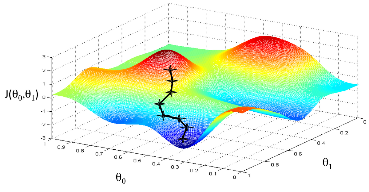
Gradient Descent Visual

Optimizers are at the heart of training deep learning models, determining how quickly and effectively a model can converge to a solution. In this article, we'll compare four popular gradient descent optimizers: Stochastic Gradient Descent (SGD), Adam, AdamW, and LAMB.

Stochastic Gradient Descent (SGD)

SGD is simple and yet a powerful optimization algorithm used to update parameters in neural networks. It approximates the gradient of the loss function with respect to the parameters using only a single or a few samples. Though it can be noisy, SGD has been successful in various applications due to its simplicity and effectiveness, especially when combined with momentum to sustain updates in relevant directions.

Adam

Adam, which stands for Adaptive Moment Estimation, combines elements from RMSprop and SGD with momentum. It calculates an adaptive learning rate for each parameter, not only considering the average of past squared gradients (as in RMSprop) but also leveraging the moving average of the gradient similar to momentum. This results in faster convergence in practice, particularly in complex systems with vast data and parameters.

AdamW

AdamW is a tweak on the original Adam optimizer that corrects its weight decay approach. Traditional weight decay regularizes the network by penalizing large weights through simple subtraction. However, in Adam, this form of weight decay conflicts with the adaptive learning rates. AdamW decouples the weight decay from the gradient updates, often leading to better generalization and stability in training.

LAMB

LAMB, short for Layer-wise Adaptive Moments optimizer for Batch training, extends the concept of adaptive learning rate to large batch situations. The distinguishing factor is its layer-wise application of normalization on the second-moment estimator. Designed for accelerating training of deep learning models with large datasets and distributed settings, LAMB facilitates higher performance without extensive hyperparameter tuning.

All these optimizers aim to minimize the loss function, but they differ in their approach to processing gradients and updating weights. SGD is straightforward but may require more iterations to converge. Adam introduces adaptivity but might lead to suboptimal solutions in some scenarios. AdamW adjusts Adam's process by addressing weight decay separately, potentially offering better training dynamics. Lastly, LAMB is designed for high-performance computing, scaling well with larger models and datasets.

Choosing the right optimizer depends on the problem at hand, dataset characteristics, and computational resources. It's crucial for practitioners to understand their nuances and apply them judiciously to achieve the best possible results in training deep neural networks.

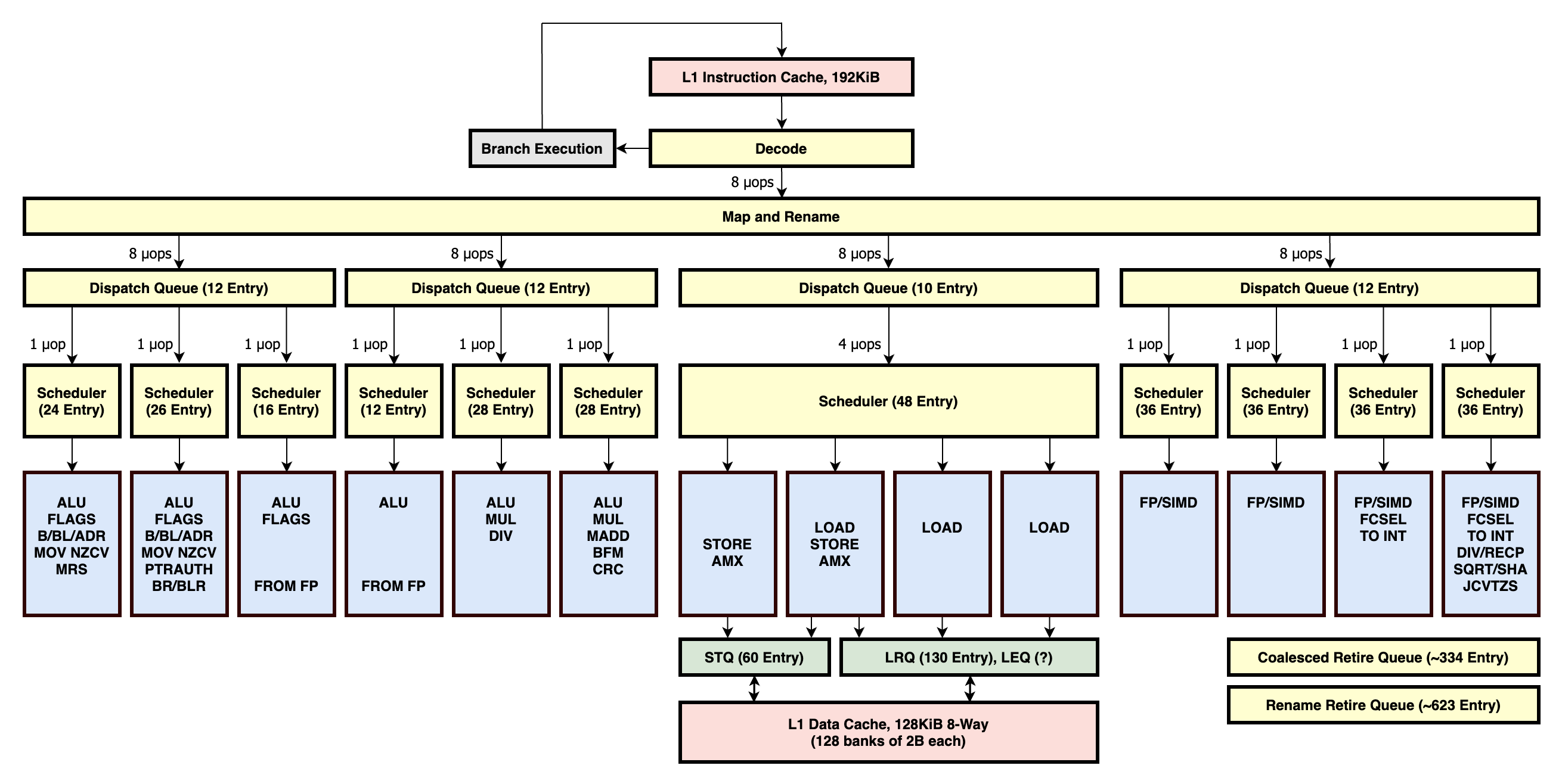
Exploring Apple Silicon Assembly: Basics and System Calls

Published: January 30th, 2024

Apple Silicon Assembly Code

The world of assembly programming is deeply fascinating. This low-level programming enables direct hardware control and efficiency, essential for performance-critical applications. Today, we delve into a simple Apple Silicon assembly code to understand its structure and system calls.

Apple Silicon, based on the ARM architecture, brings a unique approach to assembly programming. Unlike traditional x86 assembly, ARM’s instruction set is known for its simplicity and clean syntax, as demonstrated in the following example:

              
.global _start
.align 2
_start:
    mov x3, #0        // Set counter to 0
    mov x4, #10       // Set comparison to 10
    b loop

loop:
    cmp x3, x4
    b.lt print
    b terminate

print:
    mov x0, #1         // Moves the value 1 into the register X0 for stdout
    adr x1, helloworld // address reference to print out hello world
    mov x2, #12         // Number of bytes to write
    mov x16, #4        // Syscall number for writing data
    svc 0              // System call
    add x3, x3, #1     // Increment counter
    b loop

terminate:
    mov x0, #0         // Exit status
    mov x16, #1        // Syscall number for exit
    svc 0   

helloworld: .ascii  "hello world\n"


This assembly code snippet for Apple Silicon demonstrates a basic loop structure with system calls. The program prints "hello world" ten times before terminating. It showcases the usage of various instructions such as 'mov', 'cmp', 'b.lt', and 'svc' which are integral to ARM’s assembly language.

The key elements to notice here include the '.global' directive, which makes the '_start' symbol visible to the linker, and the '.align' directive, ensuring that the _start is aligned on a 4-byte boundary. This alignment is critical for performance optimization in some architectures.

System calls are particularly noteworthy in this example. The 'svc 0' instruction triggers a system call, which in this case, is used for writing to the standard output or exiting the program. The registers 'x0', 'x1', 'x2', and 'x16' play specific roles in setting up these system calls, adhering to the conventions of the ARM architecture.

Understanding such assembly code on Apple Silicon is not just an academic exercise but a practical skill for developers working on performance-sensitive applications. It offers insights into the low-level workings of modern ARM-based processors and is a stepping stone for those aspiring to delve deeper into system-level programming on Apple platforms.

Neural Networks: Parallelization via Mini-Batching

Published: January 29th, 2024

Mini-Batch Processing in Neural Networks

Mini-batching is a powerful technique in neural networks that involves processing multiple data samples simultaneously, significantly boosting computational efficiency and enabling parallelism in both forward and backward passes.

Typically, in neural networks, data is processed one sample at a time. However, mini-batching combines several samples into a single batch, allowing the network to process multiple samples concurrently. This approach not only speeds up the training process but also helps in optimizing the generalization performance of the model.

One key aspect of mini-batching is its impact on backpropagation and the forward pass. When a mini-batch is passed through the network, the forward pass computes outputs for all samples in the batch simultaneously. Similarly, during backpropagation, gradients are calculated for each sample in the batch and then averaged, reducing the variance in gradient estimates and often leading to more stable and faster convergence.

Let's explore this concept with a simplified code example:

              
    def mini_batch_forward_backward(network, input_batch, target_batch):
        # Forward pass
        activations = forward_pass(network, input_batch)
  
        # Calculate loss
        loss = compute_loss(activations, target_batch)
  
        # Backward pass
        gradients = backward_pass(activations, target_batch)
  
        # Update network parameters
        update_network(network, gradients)
  
        return loss


This pseudo-code illustrates the mini-batch processing within a neural network. During the forward pass, 'input_batch' contains multiple samples, and the 'forward_pass' function computes activations for each of them. The loss is then computed based on the difference between these activations and the target batch. During the backward pass, gradients are calculated for the entire batch, and the network parameters are updated accordingly.

Mini-batching not only accelerates the training process but also leverages modern computing architectures, such as GPUs, more effectively. GPUs are particularly well-suited for parallel computations, making them ideal for processing large batches of data simultaneously.

Neural Networks: Matrix Multiplication Part IX

Published: January 28th, 2024

3D Tensor Multiplication Diagram

Delving into tensor multiplication within neural networks reveals dimension broadcasting plays a pivotal role. Unlike matrix dimensions that engage directly in the multiplication process, batch dimensions serve as an organizational axis around which broadcasting rules apply.

In many deep learning frameworks, tensors are employed to represent not just individual data points but entire batches of them. These batch dimensions allow for parallel processing and efficiency gains. However, tensor operations like multiplication between these batched data structures require adherence to specific broadcasting rules - rules that primarily revolve around matching batch sizes.

The distinction is clear; while the inner matrix dimensions must adhere to the conventional rules of matrix multiplication (e.g., the second dimension of the first matrix must match the first dimension of the second matrix), the batch dimension follows the broadcasting rule: It either matches or is of size one, allowing expansion to match the corresponding batch dimension of another tensor.

To illustrate this concept, consider a neural network layer that processes multiple tensors simultaneously. The input tensor might have a shape that includes a batch dimension, and the following dimensions represent the actual matrix data. In contrast, weight matrices may lack an explicit batch dimension, yet, through broadcasting, they effortlessly align with the input tensor's batch dimension for successful multiplication.


      def tensor_multiplication(tensor1, tensor2):
          # Assuming tensor1 has dimensions (batch_size, i, j) where 'batch_size' is the batch dimension
          # and tensor2 has dimensions (i, k) with implicit single 'batch' dimension due to broadcasting
          result = np.zeros((tensor1.shape[0], tensor1.shape[1], tensor2.shape[1]))
          
          # Iterate over the dimensions ensuring batch sizes align through broadcasting
          for batch in range(tensor1.shape[0]):
              for i in range(tensor1.shape[1]):
                  for j in range(tensor2.shape[1]):
                      # Execute dot product respecting the broadcasting rules for batch dimensions
                      result[batch, i, j] = np.dot(tensor1[batch, i, :], tensor2[i, j])
    
          return result


This 'tensor_multiplication' function clarifies the interaction between batch dimensions and matrix dimensions during tensor multiplication. Here, broadcasting rules seamlessly permit multiplication across different batch sizes by inherently treating the non-batch dimensions of matrices as broadcastable along the larger batch dimension of the input tensor.

Summarily, understanding the dichotomy between batch and matrix dimensions in tensor operations is critical for developing and troubleshooting neural network architectures. The batch dimensions rely on broadcasting to synchronize across tensors, ensuring coherent data processing, while matrix dimensions engage in multiplication according to linear algebraic principles.

Neural Networks: Matrix Multiplication Part VIII

Published: January 26th, 2024

3D Tensor Multiplication Diagram

While many are familiar with matrix multiplication, tensor multiplication extends this concept into higher dimensions playing a crucial role in handling complex data structures in deep learning models.

Tensors, or multi-dimensional arrays, are the backbone of data representation in neural network architectures. Understanding how tensors interact through multiplication is fundamental for developing and optimizing neural networks.

Tensor multiplication is an extension of traditional matrix multiplication into higher dimensions. For instance, in 3-dimensional tensors, this involves performing matrix multiplication across slices or sub-tensors of the original tensors. The process requires careful alignment of the dimensions and understanding how these high-dimensional data structures interact.

              
  def tensor_multiplication(tensor1, tensor2):
      # Assuming tensor1 has dimensions (i, j, k) and tensor2 has dimensions (k, m, n)
      # Initialize the result tensor
      result = np.zeros((tensor1.shape[0], tensor1.shape[1], tensor2.shape[1], tensor2.shape[2]))
      
      # Iterate over the dimensions
      for i in range(tensor1.shape[0]):
          for j in range(tensor2.shape[1]):
              for k in range(tensor1.shape[1]):
                  result[i, :, j, :] += np.dot(tensor1[i, k, :], tensor2[k, j, :])
      return result


The provided 'tensor_multiplication' function is an example of how 3D tensor multiplication can be implemented in Python. The function handles tensors with specific dimensions and performs dot product operations across the relevant slices, resulting in a new 4D tensor.

This operation is fundamental in neural network computations, particularly in layers like convolutional layers where multi-dimensional data is the norm. By iterating through dimensions and performing matrix multiplications on slices, it captures complex relationships within the data.

Tensor multiplication is not just a mathematical curiosity but a practical necessity in neural networks. It allows for the manipulation and transformation of high-dimensional data, enabling neural networks to learn from complex and voluminous datasets. This understanding is crucial for anyone delving into deep learning and advanced neural network architectures.

Exploring Double vs. Single Precision in Computing

Published: January 18th, 2024

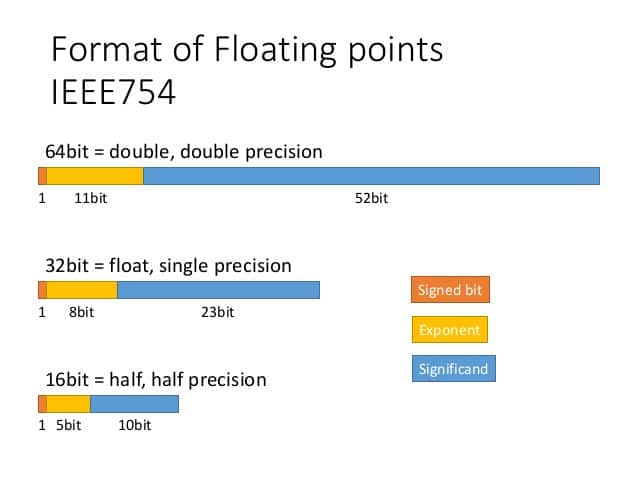
IEEE 754 Double Floating Point Format Diagram

In the realm of computing, precision is a key aspect that determines the accuracy and performance of numerical calculations. This article explores the differences between double precision and single precision numbers, emphasizing their impact in various computing scenarios, including scientific computations, graphics processing, and machine learning.

Both single and double precision numbers refer to the format in which floating-point numbers are stored in computer memory. Single precision occupies 32 bits, providing about 7 decimal digits of accuracy. Double precision, on the other hand, uses 64 bits, offering approximately 15 decimal digits of accuracy.

Single precision is often used in applications where a large range of numbers needs to be stored but where the precision of each number is not crucial. Examples include certain graphics processing tasks and large 3D models where space and processing speed are more critical than exact accuracy.

Double precision, with its higher accuracy, is essential in scientific calculations, financial applications, and other fields where minute differences can lead to significant changes in outcomes. It provides a more extensive range and greater precision, reducing the errors in calculations, particularly in iterative processes where errors can accumulate.

One of the trade-offs between single and double precision is performance versus storage. Single precision operations are generally faster and require less memory, making them suitable for high-performance computing where speed is crucial. In contrast, double precision operations, while more accurate, consume more memory and processing power.

In modern computing environments, especially in GPUs and specialized hardware for machine learning, there is a constant push for faster computations. The choice between single and double precision plays a critical role in balancing speed and accuracy. For instance, neural networks often use single precision or even lower precision formats for faster training and inference.

The choice between single and double precision can significantly impact the outcomes in different applications. In machine learning, for example, using single precision might speed up training but can introduce accuracy issues in the final model. In contrast, scientific simulations that model complex physical phenomena often require double precision to ensure the fidelity of the results.

Ultimately, the decision to use single or double precision depends on the specific requirements of the application, including the need for speed, storage efficiency, and accuracy. Understanding the strengths and limitations of each can guide developers and researchers in making informed choices that best suit their computational needs.

Neural Networks: Matrix Multiplication Part VII (Blocking)

Published: January 12th, 2024

Blocked Matrix Multiplication Diagram

Matrix multiplication is not only a foundational operation in linear algebra but also a critical component in high-performance computing and machine learning. In this article, we delve into an optimization technique known as 'blocking' and demonstrate its significant performance benefits in matrix multiplication.

Matrix multiplication, especially for large matrices, can be computationally intensive and time-consuming. Optimizing this process is crucial in applications where speed and efficiency are paramount, such as in large-scale data analysis and deep learning algorithms.

Understanding Blocking in Matrix Multiplication

Blocking is a technique used to improve the performance of matrix multiplication by optimizing memory usage, particularly the CPU cache. It involves dividing the matrices into smaller sub-matrices or blocks, and then performing the multiplication on these blocks. This method helps in keeping the frequently accessed data within the CPU cache, reducing the time-consuming memory accesses.

                
def blocked_matmul(matrix1, matrix2, block_size):
    # Initialize the result matrix
    result = np.zeros((len(matrix1), len(matrix2[0])))
    
    # Iterate over the matrices in blocks
    for i in range(0, len(matrix1), block_size):
        for j in range(0, len(matrix2[0]), block_size):
            for k in range(0, len(matrix2), block_size):
                # Compute multiplication for each block
                for i1 in range(i, min(i + block_size, len(matrix1))):
                    for j1 in range(j, min(j + block_size, len(matrix2[0]))):
                        for k1 in range(k, min(k + block_size, len(matrix2))):
                            result[i1][j1] += matrix1[i1][k1] * matrix2[k1][j1]
    return result


The 'blocked_matmul' function implements matrix multiplication with blocking. The function takes two matrices and a block size as input. It initializes the result matrix and then iterates over the input matrices in blocks determined by the given block size.

For each block, the function performs multiplication in a manner similar to the standard matrix multiplication, but restricted to the elements within the current blocks. This way, it ensures that the working set of data stays within the CPU cache, significantly enhancing the multiplication performance, especially for large matrices.

Performance Benefits of Blocking

Blocking substantially improves the efficiency of matrix multiplication. By reducing cache misses and minimizing memory access overhead, it speeds up the computation. This is particularly noticeable in large matrix operations common in scientific computing and machine learning. Studies and benchmarks show that blocked matrix multiplication can outperform traditional methods, especially on modern processors with complex memory hierarchies.

Understanding Matrix Multiplication in Python

Published: January 12th, 2024

Matrix Multiplication Diagram

Matrix multiplication, a fundamental concept in linear algebra, plays a crucial role in various mathematical and computational applications including neural networks. In this article, we will explore the inner workings of a custom matrix multiplication function I wrote and understand how it performs this essential mathematical operation.

Matrix Multiplication as a Linear Transformation

At its core, matrix multiplication can be thought of as a tool for performing linear transformations. When we multiply matrices, we are effectively combining multiple linear transformations into one. This process enables us to manipulate data points in multidimensional space, making it a powerful technique used in various computational tasks.

Custom Matrix Multiplication Function

Let's dive into the Python code for a custom matrix multiplication function:

            
    def matmul(matrix1, matrix2):
        # Check if the number of columns in matrix1 matches the number of rows in matrix2
        if len(matrix1[0]) != len(matrix2):
            raise ValueError("Number of columns in the first matrix must be equal to the number of rows in the second matrix.")
        
        # Determine the data type of the result based on the data types of input matrices
        result_dtype = np.result_type(matrix1, matrix2)
    
        # Initialize the result as a NumPy array filled with zeros and the determined data type
        result = np.zeros((len(matrix1), len(matrix2[0])), dtype=result_dtype)
    
        # Matrix 2 x traversal
        for m2x in range(len(matrix2[0])):
            # Matrix1 y traversal
            for m1y in range(len(matrix1)):
                # Matrix 1 x traversal
                dp = 0
                for m1x in range(len(matrix1[m1y])):
                    dp += matrix1[m1y,m1x] * matrix2[m1x,m2x]
                result[m1y,m2x] = dp
    
        return result


The 'matmul' function takes two matrices, 'matrix1' and 'matrix2,' as input. Before performing the multiplication, it checks if the number of columns in 'matrix1' matches the number of rows in 'matrix2,' ensuring compatibility for matrix multiplication.

The function then determines the data type of the result matrix based on the data types of the input matrices, ensuring consistency in the result data.

Next, it initializes the result matrix, 'result,' as a NumPy array filled with zeros, with the determined data type, to store the output of the multiplication.

The function proceeds with the multiplication process, traversing 'matrix2' column by column ('m2x') and 'matrix1' row by row ('m1y'). Within these loops, a dot product ('dp') is calculated for each element of the result matrix. The dot product is computed by iterating through the elements of 'matrix1' and 'matrix2' and summing their products.

Finally, the calculated dot product ('dp') is assigned to the corresponding element in the 'result' matrix, completing the matrix multiplication.

Metric Prefixes

Published: January 11th, 2024

Computer Chips Image

Metric prefixes are not just a matter of numbers; they are the keystones in understanding computing power, memory capacity, and data measurement. Just as the cosmos is vast, so is the field of computing, where the use of metric prefixes helps us navigate the immensity of digital space.

From kilobytes to petabytes, each metric prefix represents a leap in magnitude, essential for accurately describing the capabilities of computers and the size of digital files. For example, knowing the difference between a megabyte (MB) and a gigabyte (GB) is crucial when evaluating storage solutions or internet bandwidth. These prefixes are not just numerical values; they are indicators of technological progression.

Furthermore, the evolution of these terms reflects the rapid advancement of technology. With the emergence of zettabytes and yottabytes, our lexicon expands to encompass the burgeoning scale of data in the modern world. Each new prefix not only quantifies size but also signifies a milestone in human innovation. As we continue to push the boundaries of what's possible in computing, our understanding and utilization of these metric prefixes will continue to evolve, painting a picture of our journey through the digital age.

The Fear of God is the Beginning of Knowledge

Published: January 7th, 2024

Neural Network Concept Image

As we marvel at the complexity of the world around us - from the intricacies of the human brain to the vastness of the cosmos - it is humbling to consider that there is an all-powerful Creator behind it all. Approaching learning with a passionate curiosity about how God designed and ordered the universe allows us to fully appreciate both His majesty and the gift of an inquisitive mind.

Rather than view education as merely a means to material ends, we can embrace the process of lifelong learning as an act of worship. The more we discover about math, science, language, and all fields of study, the more we uncover about God's nature reflected through creation. This knowledge should inspire awe and gratitude.

Cultivating an insatiable curiosity to comprehend the breadth of God's craftsmanship is a path to deeper communion with Him. Through devoted inquiry, we begin to grasp the beauty of His intentional design. Such understanding nourishes the soul and provides a foundation for living purposefully in light of eternal truth.

Neural Networks #16: Matrix Multiplication Part VI

Published: January 5th, 2024

Neural Network Concept Image

The role of Single-Precision General Matrix Multiply (SGEMM), is integral to autograd efficiency and performance. SGEMM, a standard routine in linear algebra, is used for multiplying matrices where data is stored in single precision floating point format. This method is highly efficient in handling the large-scale computations required by neural networks.

Modern autograd engines, tools designed to automatically compute the derivatives of tensor operations in neural networks, heavily rely on SGEMM. This is due to the intensive nature of backpropagation, a method used for training neural networks. Backpropagation involves calculating gradients, or changes, across matrices, to update the network’s weights. Efficient matrix multiplication, as facilitated by SGEMM, is essential for this process, ensuring rapid and accurate updates.

Furthermore, SGEMM's significance extends beyond basic matrix operations. It optimizes the utilization of hardware resources, like GPUs, enabling neural networks to process vast amounts of data at remarkable speeds. This optimization is crucial for deep learning applications where real-time processing and high computational power are essential.

Neural Networks #16: Matrix Multiplication Part V

Published: January 4th, 2024

Neural Network Concept Image

One of the most remarkable aspects of neural networks is their ability to handle inputs of varying dimensions - from one-dimensional data in time-series to multi-dimensional data like images. This versatility is enabled by the network's capacity to transform these inputs to align with the dimensions of its layers, making neural networks suitable for a wide range of applications.

Central to spatial transformation within neural networks are weight matrices. Each layer in a network possesses a weight matrix that interacts with incoming data. When input data is fed into the network, it undergoes a series of transformations through these weight matrices, changing its dimensionality and representation to suit the network's architecture.

Neural Networks #16: Matrix Multiplication Part IV

Published: January 4th, 2024

Neural Network Concept Image

Dimensionality reduction refers to the process of reducing the number of random variables under consideration, by obtaining a set of principal variables. In simpler terms, it's about simplifying the data without losing its essential characteristics. This is especially important in dealing with high-dimensional data such as images, videos, and large-scale datasets common in machine learning.

The dot product, a simple yet powerful mathematical operation, is at the heart of this process. When used in conjunction with weights within neural networks, it helps in mapping the high-dimensional input data to a lower-dimensional space. This mapping is crucial for several reasons, including enhancing the interpretability of the data, reducing computational load, and improving model performance by mitigating the risk of overfitting.

Through dimensionality reduction, neural networks can focus on the most relevant aspects of the data, filtering out noise and irrelevant information. This focus not only speeds up the learning process but also enhances the network's ability to generalize from the training data to new, unseen data. The network learns to identify and leverage the underlying patterns and structures within the data, which are often lost in the maze of high-dimensional space.

The implications of this are vast, spanning various domains from image and speech recognition to natural language processing. In each of these fields, the ability to reduce dimensionality effectively allows for more efficient processing and analysis, leading to more accurate and reliable outcomes.

Neural Networks #16: Matrix Multiplication Part III

Published: January 3rd, 2024

Neural Network Concept Image

One of the most crucial aspects of matrix multiplication is the summation of products. This process is not just a mathematical rule, but a fundamental mechanism that combines multiple dimensional effects into a single outcome. It's key to understanding the geometrical and practical implications of linear transformations in linear algebra.

Why Summation Matters

Summation in matrix multiplication is essential for fully applying a multidimensional transformation. Without summing these products, you would only capture a partial view of how each dimension influences the others, missing the complete transformation effect. This summation integrates the different interactions between dimensions, providing a comprehensive transformation.

From a geometric viewpoint, without the summation of these products, you wouldn't fully capture the effects of transformation, such as rotation and scaling in multidimensional space. This is crucial in applications like physics, engineering, and computer graphics, where understanding spatial transformations is key.

Neural Networks #17: Matrix Multiplication Part II

Published: January 2nd, 2024

Matrix Multiplication Diagram

Matrix multiplication, a pivotal concept in linear algebra, is effectively a multidimensional linear transformation of data possessing linear properties. This operation is not only fundamental in mathematics but also forms the backbone of various applications in engineering, physics, and computer science, particularly in fields like machine learning and computer graphics.

Matrix Multiplication as Linear Transformation

At its core, a matrix can be seen as a tool for linear transformation. When we multiply matrices, we are essentially combining multiple linear transformations into one. This process allows us to manipulate data points in multidimensional space, making it a powerful technique for various computational operations.

Matrix Multiplication in Python with NumPy

              
      # Import NumPy
      import numpy as np
  
      # Define two matrices
      A = np.array([[1, 2], [3, 4]])
      B = np.array([[5, 6], [7, 8]])
  
      # Perform matrix multiplication
      C = np.dot(A, B)


This Python example demonstrates basic matrix multiplication using NumPy, a popular numerical computing library. Here, np.dot() is used to multiply two matrices, A and B, resulting in a new matrix C.

Understanding the Linear Nature of Matrix Multiplication

Each element of the product matrix is a linear combination of elements from the row of the first matrix and the column of the second matrix. This reflects the linear nature of the transformation, where each output dimension is influenced by all input dimensions in a linear manner.

Applications in Various Fields

Matrix multiplication's ability to handle multidimensional linear transformations makes it invaluable in fields like image processing, where transformations of pixel data are common, and in machine learning, where it's used in algorithms for data classification and regression.

Neural Networks #16: Matrix Multiplication Part I

Published: December 30, 2023

Neural Network Concept Image

Matrix multiplication is a cornerstone operation in neural networks, particularly in layers like fully connected and convolutional layers. It involves the dot product of matrices, which represents the weighted sum of inputs.

Matrix Multiplication in Python with NumPy

              
      # Import NumPy
      import numpy as np
  
      # Define two matrices
      A = np.array([[1, 2], [3, 4]])
      B = np.array([[5, 6], [7, 8]])
  
      # Perform matrix multiplication
      C = np.dot(A, B)


This code snippet shows a basic example of matrix multiplication using NumPy's dot function.

Memory Considerations in Matrix Multiplication

From a hardware perspective, matrix multiplication can be memory-intensive, especially for large matrices. The efficiency of matrix multiplication depends on how data is stored and accessed in memory.

Optimizing Memory Usage

Optimizing memory usage involves techniques like using data types with lower memory footprints and leveraging hardware acceleration (like GPUs) where matrix operations can be parallelized.

Impact on Neural Network Performance

Efficient matrix multiplication directly impacts the speed and performance of neural networks. It reduces training time and allows for more complex models to be trained on larger datasets.

AGI: The Pursuit of Deep Beauty in Transcendent Intelligence

Published: January 2, 2024

Artificial Intelligence Concept Image

As we stand on the brink of creating Artificial General Intelligence (AGI), it's important to reflect on the motivations behind this monumental human endeavor and its implications.

The pursuit of AGI is not just a technological milestone; it's a quest driven by our longing to witness deep beauty and transcendent complexity. This innate desire mirrors the biblical acknowledgment of the complexity and beauty in God’s creation (Psalm 19:1). In creating AGI, humans aspire to mimic, in a small way, the creative capabilities bestowed upon them as bearers of the Imago Dei - the Image of God.

The development of AGI serves as a testament to human creativity, a gift from the Creator. However, it also highlights our limitations. Unlike God, who is omniscient and omnipotent, our creations, however sophisticated, are finite and fallible. AGI, while potentially reaching or surpassing human intelligence in certain aspects, will always lack the divine attributes of God, such as His perfect wisdom, justice, love (Isaiah 55:8-9), and even His intelligence.

In our quest to create a superintelligence, it's crucial to recognize that we are already in the presence of an ultimate superintelligence - God Himself. Yahweh, the God of Abraham, Isaac, and Jacob, embodies an intelligence and wisdom far beyond human comprehension (Romans 11:33-36). In the pursuit of AGI, we must not lose sight of this profound truth and must maintain a posture of humility and reverence towards our Creator.

For those of us who are researchers in the AI space and who are Christians, as we advance in the realm of AI towards AGI, we must balance our technological pursuits with theological and ethical understanding. We must ensure that our endeavors honor God and reflect our stewardship of His creation (Genesis 1:28). This means developing AI responsibly, ethically, and in ways that uphold the dignity and value of all human life, as created in God's image.

In conclusion, while the development of AGI is a remarkable testament to human creativity and intelligence, it also serves as a reminder of our finite nature and the infinite wisdom and power of God. As we continue to explore and create, let us do so with a sense of wonder at the greater intelligence and beauty found in God, and with a commitment to reflecting His glory in all that we do.

Neural Networks #15: Computation Graphs

Published: December 30, 2023

Neural Network Concept Image

In this article, we explore the intricacies of computation graphs and automatic differentiation, which are pivotal in training neural networks. Understanding these concepts is crucial for effectively leveraging machine learning frameworks like PyTorch and TensorFlow.

What is a Computation Graph?

A computation graph is a representation of the operations and variables involved in calculating a function. In neural networks, this graph delineates how different operations, like matrix multiplication and activation functions, combine to produce the final output.

Example: Simple Neural Network Operation

            
    # Python example: Defining a simple operation
    w = 2    # Weight
    x = 3    # Input
    b = 4    # Bias
  
    y = w * x  # Operation 1
    z = y + b  # Operation 2


This code snippet represents a basic computation with two operations. The corresponding computation graph would have nodes for `w`, `x`, `b`, `y`, and `z`, with edges connecting them to represent the operations.

Intermediate Values in Forward Pass

During the forward pass, intermediate values (like `y` in our example) are computed and stored. These values are crucial for efficiently computing gradients in the backward pass.

Backpropagation and Gradient Calculation

In backpropagation, gradients of the loss with respect to each parameter are calculated using the chain rule. This process relies heavily on the intermediate values stored during the forward pass.

            
    # Hypothetical backward pass calculation
    dL_dz = 1  # Derivative of loss with respect to z
    dL_dy = dL_dz * 1  # Since z = y + b
    dL_dw = dL_dy * x  # Using stored value of x


This example shows how gradients are computed. The stored value of `x` is reused, avoiding redundant computation.

Efficiency and Importance in Neural Networks

Automatic differentiation and computation graphs provide a systematic and efficient way of calculating gradients, which is essential for training neural networks. By storing intermediate values, these frameworks significantly reduce computational overhead, especially in deep and complex networks.

Conclusion

Understanding computation graphs and automatic differentiation is fundamental for anyone looking to delve into neural network development. These concepts are at the core of efficient gradient computation, enabling the training of sophisticated models in modern machine learning frameworks.

Neural Networks #14: Delineating the Frontend from the Backend

Published: December 30, 2023

Neural Network Concept Image

In the realm of neural network development, the distinction between Python's frontend and backend plays a crucial role in efficiency and performance. This article explores how neural network frameworks utilize different backends for optimal speed and performance, while maintaining an accessible Python frontend.

The Role of Python Frontend

Python, known for its simplicity and readability, is predominantly used as the frontend language in neural network frameworks. It allows developers to easily define models, set up training loops, and perform data manipulation. The frontend handles the user interface part of the framework, translating high-level Python commands into backend instructions.

          
  # Python Frontend Example: Defining a model in PyTorch
  import torch.nn as nn

  class SimpleNN(nn.Module):
      def __init__(self):
          super(SimpleNN, self).__init__()
          self.linear = nn.Linear(10, 5)

      def forward(self, x):
          return self.linear(x)


Understanding the Backend

The backend is where the heavy lifting occurs. It's responsible for executing the computations defined by the frontend in an optimized manner. Typically written in performance-oriented languages like C++ or CUDA, the backend handles tasks like tensor operations, memory management, and execution of complex mathematical operations.

Compilation to Machine Code for Optimization

For greater performance, Python code is often compiled down to machine code. Frameworks use various techniques like Just-In-Time (JIT) compilation or Ahead-Of-Time (AOT) compilation. These methods convert high-level Python instructions into optimized, low-level machine code, significantly speeding up the execution.

          
  # JIT Compilation Example in PyTorch
  model = SimpleNN()
  scripted_model = torch.jit.script(model)


Different Backends for Different Needs

Neural network frameworks often support multiple backends. For instance, TensorFlow can use its own backend or leverage others like NVIDIA's cuDNN for GPU acceleration. PyTorch uses its native backend and integrates with libraries like Intel MKL for optimized CPU performance. This flexibility allows the framework to be highly efficient on various hardware platforms.

By separating concerns, neural network frameworks offer the best of both worlds: ease of use and high performance. The Python frontend provides an accessible interface for model development, while the optimized backend ensures efficient computation, making it possible to train complex models in less time.

Key Takeaways

Understanding the interplay between frontend and backend in neural network frameworks empowers developers to effectively utilize these tools for building sophisticated models.

Neural Networks #13: Weight Initialization with He and Xavier

Published: December 29, 2023

Neural Network Concept Image

Proper weight initialization is crucial for training deep neural networks effectively. Two popular techniques for initialization are the He initialization and Xavier initialization methods. This article will provide an overview of these methods and why weight initialization matters.

The Problem of Vanishing/Exploding Gradients

During training, gradients need to flow properly backwards through the network layers. If weights are poorly initialized, gradients may shrink rapidly (vanish) or grow out of control (explode), preventing effective learning. This problem gets worse with more layers.

He Initialization

He initialization was proposed specifically for layers using a ReLU activation function. It draws random weights from a distribution with a standard deviation of √2/nl, where nl is the number of inputs feeding into that layer.

              
  import numpy as np

  num_inputs = 128
  num_neurons = 256

  stddev = np.sqrt(2/num_inputs)
  weights = np.random.normal(loc=0.0, scale=stddev, size=[num_inputs, num_neurons]) 


This ensures signal and gradient flow remains normalized across layers using ReLU. Otherwise, signal may shrink towards zero, while gradients shrink towards zero much faster.

Xavier Initialization

Xavier initialization is more general and works for other activation functions like tanh. Weights are initialized from a distribution with standard deviation of √1/nl.

              
  import numpy as np

  num_inputs = 128
  num_neurons = 256
  
  stddev = np.sqrt(1./num_inputs)
  weights = np.random.normal(loc=0.0, scale=stddev, size=[num_inputs, num_neurons])


This maintains variance of signals and gradients across layers for tanh networks. The key difference from He initialization is accounting for the non-linear saturating behavior of activations like tanh.

Why Weight Initialization Matters

In summary, proper weight initialization helps:

Understanding these techniques allows one to properly train deeper and more complex neural network architectures.

Neural Networks #12: Understanding the Adam Optimizer

Published: December 28, 2023

Neural Network Concept Image

The Adam (Adaptive Moment Estimation) optimizer has emerged as a popular algorithm for training neural networks. It combines ideas from two other optimization algorithms - AdaGrad and RMSProp - to provide an efficient and effective method for adjusting network weights.

How Adam Works:

Adam maintains two sets of estimates for each network parameter: the first moments (the mean of the gradients) and the second moments (the uncentered variance). These are updated at each step with the new gradients.

One of Adam's key features is its adaptive learning rate. Unlike traditional methods that use a single learning rate for all weight updates, Adam adjusts the rate based on the first and second moments. This allows for a more nuanced and effective approach to converging on optimal weights.

Benefits of Adam:

Adam stands out for its efficiency in large-scale data and parameter settings. It is particularly useful in situations where gradients are sparse or noisy, making it a preferred choice for many deep learning applications.

Additionally, Adam's adaptive nature makes it less sensitive to hyperparameter settings, particularly the initial learning rate, compared to other optimizers.

Despite its strengths, Adam is not a silver bullet. It may not always converge to the global minimum for non-convex optimization, a common scenario in deep learning. Practitioners often couple Adam with strategies like learning rate annealing or gradient clipping to enhance its performance.

The Adam optimizer represents a significant advancement in training neural networks, offering a balance between efficiency and effectiveness. It continues to be a valuable tool in the machine learning practitioner's toolkit.

Neural Networks #11: The Challenge of Exploding Gradients

Published: December 27, 2023

Neural Network Concept Image

The phenomenon of exploding gradients presents a significant challenge. This occurs when the gradients used in training algorithms become excessively large, leading to unstable training processes and hindering model convergence. Understanding and mitigating exploding gradients is crucial for the effective training of deep neural networks.

Understanding Exploding Gradients:

          
    def calculate_gradient(loss, weights):
      return 2 * loss * weights
        

Exploding gradients often occur in networks with many layers. During backpropagation, gradients of the loss function with respect to the network's parameters are calculated. If these gradients are large, they result in large updates to the network's weights, potentially leading to an unstable training process where the weights oscillate or diverge.

Several factors contribute to this problem, including deep network architectures, improper initialization of weights, and unsuitable choice of the learning rate. Additionally, certain activation functions can exacerbate the issue, particularly when their derivatives can take on large values.

The Impact of Network Architecture:

Deep networks are particularly prone to exploding gradients due to the multiplicative effect of gradients through many layers. The more layers a network has, the more the gradient can exponentially increase as it backpropagates through each layer.

This issue is more pronounced with certain activation functions and network configurations. For instance, networks using the ReLU activation function can be susceptible to exploding gradients if the weights are not properly initialized or if the learning rate is too high.

Mitigation Strategies:

To combat exploding gradients, various strategies can be employed. Gradient clipping is a common technique where the gradient is scaled down if it exceeds a certain threshold. Additionally, employing batch normalization can help in stabilizing the learning process by normalizing the inputs to each layer.

Proper initialization of weights and careful selection of the learning rate are also crucial in preventing this issue. Techniques like Xavier or He initialization can provide a good starting point for weights, helping to keep the gradients in a reasonable range during training.

Understanding and addressing exploding gradients is essential for building robust and effective neural networks. By acknowledging and mitigating this challenge, AI practitioners can ensure smoother training processes and more accurate models.

Neural Networks #10: Exploring the Power of Batch Normalization

Published: December 26, 2023

Neural Network Concept Image

Batch Normalization is a fundamental technique in the world of deep learning that plays a crucial role in training deep neural networks effectively. In this article, we'll dive into the concept of Batch Normalization, its benefits, and how it enhances the training process of neural networks.

Understanding Batch Normalization

Batch Normalization, often abbreviated as BatchNorm or BN, is a technique used to normalize the input to each layer of a neural network within a mini-batch of data. The primary goal is to ensure that the activations have a consistent distribution throughout training, which leads to faster and more stable convergence.

The Benefits of Batch Normalization

Batch Normalization offers several advantages:

How Batch Normalization Works

Batch Normalization operates as follows:

  1. Calculate the mean and standard deviation of each feature (channel) within the mini-batch.
  2. Normalize the activations for each feature, making them have a mean of approximately 0 and a standard deviation of approximately 1.
  3. Learnable Parameters: Introduce learnable scaling and shifting parameters per feature to allow the network to adapt to the normalized activations.

Integration into Neural Networks

Batch Normalization is typically inserted after the linear transformation (e.g., weights and biases) and before the non-linear activation function in each layer of a neural network. It can be used in various network architectures, including convolutional neural networks (CNNs) and feedforward networks.

Conclusion

Batch Normalization is a powerful technique that revolutionized the training of deep neural networks. Its ability to stabilize training, accelerate convergence, and improve generalization makes it a fundamental tool in modern deep learning. Understanding BatchNorm and its integration into neural networks is key for practitioners looking to build effective and efficient deep learning models.

Neural Networks #9: Understanding Backpropagation and the Chain Rule

Published: December 26, 2023

Neural Network Concept Image

One of the key concepts in neural network training is backpropagation, a method that involves the application of the chain rule from calculus to adjust the network's parameters (weights and biases) based on the error in its predictions. This article will explore this fundamental concept and how it enables neural networks to learn from data.

Understanding the Basics of Backpropagation

Backpropagation is an algorithm used for training neural networks. It calculates the gradient of the loss function with respect to each weight in the network by applying the chain rule, a basic principle in calculus. This process is crucial for updating the weights in a way that minimizes the loss, thereby improving the model's predictions.

The Role of the Chain Rule

The chain rule allows us to differentiate composite functions. In the context of neural networks, the output is a composite function of the weights and biases. The chain rule helps in breaking down the derivative of the loss function with respect to the weights into simpler parts, making it computationally feasible to calculate these gradients.

Code Example: Implementing Backpropagation

Let's look at a simplified code example that demonstrates the backpropagation process:

                
      import numpy as np
      
      # A simple example of a neural network layer
      class Layer:
          def __init__(self, input_size, output_size):
              self.weights = np.random.randn(input_size, output_size) * 0.1
              self.bias = np.zeros(output_size)
      
          def forward(self, input):
              return np.dot(input, self.weights) + self.bias
      
      # Example backpropagation for a single layer
      def backpropagate(layer, input, output_gradient):
          # Gradient with respect to the weights
          weight_gradient = np.dot(input.T, output_gradient)
      
          # Gradient with respect to the input (for previous layer)
          input_gradient = np.dot(output_gradient, layer.weights.T)
      
          # Update weights and biases here (not shown for simplicity)
          # ...
      
          return weight_gradient, input_gradient
      
      # Example usage
      layer = Layer(3, 2)
      input = np.random.randn(1, 3)
      output_gradient = np.random.randn(1, 2)  # Gradient from the next layer or loss function
      weight_gradient, input_gradient = backpropagate(layer, input, output_gradient)
              

In this example, the backpropagate function takes a layer, an input, and an output gradient. It calculates the gradient with respect to the layer's weights and the gradient with respect to the input (which is passed back to the previous layer).

Conclusion

Backpropagation and the chain rule form the backbone of neural network training. By understanding these concepts, one can appreciate how neural networks are able to learn complex patterns in data and make predictions. It's a fascinating example of how a simple mathematical principle can be applied to enable sophisticated machine learning algorithms.

Neural Networks #8: Understanding the Difference Between MSE and Its Gradient

Published: December 26, 2023

Neural Network Image

Here's the problem:

When training neural networks, two concepts that often cause confusion are Mean Squared Error (MSE) and the gradient of MSE. Both are crucial in the context of machine learning, especially in regression tasks. Understanding the distinction between these two is key to grasping how neural networks learn.

MSE as a Performance Measure:

MSE is a popular loss function used in regression problems. It measures the average squared difference between the actual and predicted values. The formula for MSE is:

                
      # Mean Squared Error calculation
      def mse(y_true, y_pred):
          return ((y_true - y_pred) ** 2).mean()
              

A lower MSE value indicates that the model's predictions are closer to the actual values, implying better performance. It's a direct measure of the model's accuracy.

Gradient of MSE in Training:

While MSE measures model performance, the gradient of MSE is used during the training process. This gradient is the derivative of the MSE with respect to the model's predictions and is crucial for the backpropagation algorithm. The gradient is calculated as follows:

                
      # Gradient of MSE
      def mse_gradient(y_true, y_pred):
          return 2 * (y_pred - y_true)
              

This gradient is used to adjust the model's weights in the direction that reduces the MSE, thereby improving the model's predictions over time.

To sum up, MSE is a metric for evaluating the accuracy of a neural network, while the gradient of MSE is a tool used in optimizing the network's weights during training. Understanding both concepts is essential for effective machine learning model development.

Neural Networks #7: Understanding Matrix Multiplication

Published: December 25, 2023

Neural Network Matrix Operations

In the fascinating world of neural networks, the magic largely happens through matrix operations. One of the fundamental operations is matrix multiplication between the input data and the weights of a layer. Understanding this process is crucial to comprehending how neural networks process information and learn.

Breaking Down the Basics

The core operation in many neural network computations is np.dot(input, weights) + bias. This operation may seem daunting at first, but it becomes clearer when broken down. The process involves taking an input matrix (where each row represents a different input sample) and a weight matrix (where each column represents weights connected to a neuron), and performing matrix multiplication.

Matrix Multiplication in Action

Let's consider an example to illustrate this. Suppose you have an input matrix with several samples, each with two features. Your weight matrix for a layer with five neurons would have two rows (for the two features) and five columns (for the five neurons). When you perform the matrix multiplication of the input and the weight matrix, you effectively compute the weighted sum of the inputs for each neuron.

Understanding Through an Example

Imagine your input is a matrix with rows like [0, 1], and your weight matrix looks something like this (simplified for illustration):

      [-0.234,  0.017, -0.009, -0.045,  0.058]
      [ 0.018, -0.068,  0.042,  0.079, -0.124]
                  
The first step in matrix multiplication is to take the first row of the input and multiply each element by the corresponding element in each column of the weight matrix, then sum these products. This operation is repeated for each row of the input, generating a row in the output matrix for each input sample.

The Significance in Neural Networks

This matrix multiplication is not just a mathematical operation; it's how each layer in a neural network processes its input. The output of this operation is then typically passed through an activation function, allowing the network to learn and model complex, non-linear relationships. This ability to handle multiple inputs at once and produce corresponding outputs is part of what makes neural networks so powerful and efficient, especially when dealing with large datasets.

Conclusion

Matrix multiplication in neural networks, exemplified by the np.dot(input, weights) operation, is a cornerstone of how these models process and learn from data. Understanding this operation provides insight into the inner workings of neural networks and is essential for anyone looking to delve into the field of machine learning and artificial intelligence.

Neural Networks #6: Batch Processing Efficiency

Published: December 25, 2023

Efficient Neural Network Batch Processing

In the world of neural networks, efficiency is key. As we dive deeper into the mechanics of these sophisticated models, one aspect stands out for its impact on computational performance: batch processing. This approach, integral to modern neural network operations, allows for the simultaneous processing of multiple data samples, greatly enhancing the efficiency of the training process.

Understanding Batch Processing

Batch processing in neural networks refers to the technique of processing multiple data samples at once, rather than individually. This is achieved through the power of matrix operations, which are at the heart of neural network computations. By arranging input data into batches, neural networks can leverage the parallel processing capabilities of modern hardware, such as GPUs, leading to significant reductions in training time.

Matrix Multiplication: The Driving Force

Consider the operation self.output = np.dot(input, self.weights) + self.bias in a neural network layer. This line exemplifies the efficiency of batch processing. Here, input is not just a single data sample but a matrix representing an entire batch of samples. The weights and biases of the network are combined with this batch through matrix multiplication and addition, respectively.

The resulting matrix multiplication between the input batch and the weights produces an output matrix where each row corresponds to a sample in the batch, and each column represents the output of one neuron for all the samples. This parallel processing is far more efficient than handling each sample individually.

Advantages of Batch Processing

Batch processing brings numerous advantages. It optimizes memory usage, as operations on matrices are generally more efficient than equivalent operations on individual vectors. It also exploits the full potential of GPU acceleration, a cornerstone in modern deep learning, where parallel processing capabilities can be fully harnessed. Furthermore, batch processing can help in achieving more stable and reliable gradient updates during training, as the updates are averaged over a batch of samples, reducing the variance inherent in single-sample updates.

Conclusion

The use of batch processing in neural networks is a testament to the marriage of advanced mathematical techniques and modern computing power. By processing data in batches, neural networks achieve a level of efficiency that is crucial for handling the vast datasets and complex models prevalent in today's machine learning landscape. This efficiency not only accelerates the training process but also opens the door to more sophisticated and computationally demanding models, driving forward the boundaries of what is possible in the realm of artificial intelligence.

Neural Networks #5: The Necessity of Linear Activation in the Output Layer with ReLU

Published: December 24, 2023

Neural Network Visualization

The architecture of neural networks is a marvel of interconnecting layers and activation functions, each playing a pivotal role in learning from data. A prevalent feature in these networks is the use of the Rectified Linear Unit (ReLU) activation function in hidden layers. Yet, when it comes to the output layer, a linear activation function often becomes necessary. Why is this the case, especially when ReLU has proven so effective?

ReLU: The Preferred Choice for Hidden Layers

ReLU, defined as f(x) = max(0, x), is favored in hidden layers for several reasons. It mitigates the vanishing gradient problem, allows for faster training, and introduces non-linearity, enabling the network to learn complex patterns. However, its very nature - outputting zero for any negative input and a linear response for positive inputs - can limit its effectiveness in the output layer for certain tasks.

Linear Activation in the Output Layer

The choice of activation function in the output layer is tightly coupled with the type of task the network is designed to perform. For regression tasks, where the prediction can be any real number, a linear activation function becomes essential. This is because ReLU can restrict the output range to non-negative numbers only, which is a significant limitation for outputs that require negative values or a wider range.

A linear activation function, essentially f(x) = x, allows the network to output values across the entire range of real numbers, accommodating the requirements of diverse regression tasks. This versatility is why, despite the predominance of ReLU in hidden layers, a linear function is often the go-to choice for the output layer in regression-based neural networks.

Combining ReLU and Linear Activation

The combination of ReLU in hidden layers and linear activation in the output layer harnesses the best of both worlds. ReLU's efficiency in learning non-linear representations through hidden layers, coupled with the unbounded output of the linear activation function, enables the network to accurately model complex, real-world problems that require a wide range of output values.

Conclusion

In summary, while ReLU is a powerful tool for hidden layers in neural networks, its limitations in the output range necessitate the use of a linear activation function for the output layer in many applications, particularly regression tasks. This strategic combination allows neural networks to effectively learn and predict across a vast range of values, showcasing the nuanced yet crucial decisions that go into designing effective neural network architectures.

Neural Networks #4: The Concept of Multidimensional Slope

Published: December 24, 2023

Complex Calculus Visualization

In the realm of neural networks and machine learning, the concept of a gradient is fundamental. However, understanding what a gradient represents in this context can be challenging. One effective way to grasp this concept is to think of it as a multidimensional slope. Let's delve into this analogy to better understand gradients and how they drive the learning process in neural networks.

What is a Gradient?

In simple terms, a gradient is a vector that points in the direction of the greatest rate of increase of a function. In the context of a one-dimensional function, this is simply the slope of the function. But neural networks operate in a high-dimensional space, where each weight and bias represents a separate dimension. So here, a gradient becomes a multidimensional slope.

Gradients as Multidimensional Slopes

Imagine a landscape with hills, valleys, and various terrains. In two dimensions, the slope at any point on this landscape tells you how steep the hill is and in which direction it's steepest. Now extend this idea to a space with many more dimensions - this is the landscape of a neural network's loss function.

Each dimension corresponds to a parameter in the network (like a weight or a bias). The gradient at any point in this multidimensional space shows the direction and steepness of the slope, telling us how the loss function changes with respect to each parameter.

Importance in Neural Networks

Why is this concept crucial? In machine learning, the goal is often to minimize a loss function, which measures how well the network performs. By understanding the gradient as a multidimensional slope, we can adjust each parameter in the direction that most reduces the loss. This process is known as gradient descent.

Backpropagation: Calculating the Gradient

The process of calculating these gradients in a neural network is known as backpropagation. It involves going backward through the network, applying the chain rule of calculus, to determine the gradient (multidimensional slope) of the loss function with respect to each parameter.

Conclusion

In conclusion, viewing gradients as multidimensional slopes offers an intuitive understanding of how neural networks learn. It illustrates the process of navigating the complex landscape of the loss function to find the path to optimal performance. This perspective not only aids in conceptual understanding but also highlights the elegant interplay between mathematics and machine learning.

Neural Networks #3: The Power of the Chain Rule in Backpropagation

Published: December 23, 2023

Complex Calculus Visualization

At the heart of every neural network's learning process is a mathematical gem known as the chain rule of calculus. This fundamental principle is key to understanding how neural networks learn from data and adjust their parameters (weights and biases) accordingly. Today, we'll unravel the mystery of the chain rule and its pivotal role in the backpropagation algorithm.

What is the Chain Rule?

In calculus, the chain rule is a formula for computing the derivative of the composition of two or more functions. Simply put, if you have a function that is composed of other functions, the chain rule helps you find the rate at which this function changes by considering the rates of change of its constituent functions.

The Chain Rule in Neural Networks:

Neural networks consist of layers of neurons, where each neuron performs computations involving activation functions. The output of each neuron depends not only on its inputs and weights but also on the outputs of neurons in the previous layer. This creates a chain of functions – a perfect scenario for applying the chain rule.

Backpropagation and Gradient Descent:

Backpropagation is the process of updating the neural network's weights in response to the error in its predictions. It involves calculating the gradient (or derivative) of the network's error with respect to each weight. Here, the chain rule comes into play. It allows us to break down the derivative into manageable parts, reflecting how each weight contributes to the error.

Once the gradients are computed using the chain rule, the gradient descent algorithm updates the weights. If a weight's gradient is positive, the weight is decreased, and if it's negative, the weight is increased. This iterative process gradually minimizes the error, improving the network's performance.

Understanding Weight Updates:

The direction and magnitude of weight adjustments are crucial. The chain rule ensures that each weight is updated in a way that most effectively reduces the overall error. This precise adjustment is key to the network's ability to learn from data and make accurate predictions.

In conclusion, the chain rule is more than just a mathematical tool; it's the backbone of learning in neural networks. By enabling efficient computation of derivatives, it empowers neural networks to learn complex patterns and relationships in data, making it a cornerstone of modern machine learning and AI.

Neural Networks #2: Exploring the Tanh Activation Function

Published: December 22, 2023

Tanh Function Visualization

The tanh (hyperbolic tangent) activation function is a core element in the neural network toolbox. Known for its mathematical elegance and practical efficiency, tanh offers unique advantages in neural network design. Unlike functions that only output positive values, tanh expands the range of possibilities by including negative outputs. Let’s delve into how tanh functions and its implications in neural network architectures.

Understanding Tanh:

          
    def tanh(x):
      return (exp(x) - exp(-x)) / (exp(x) + exp(-x))
        

Tanh is a scaled version of the sigmoid function. It squashes the input values to be within the range of -1 and 1. This characteristic makes it suitable for scenarios where the model needs to represent data that naturally falls within this range or when negative outputs are as significant as positive ones.

An advantage of tanh is its zero-centered nature, making optimization easier and often leading to faster convergence during training. Unlike functions that only output positive values, tanh’s ability to output negative values allows for more dynamic adjustments during the learning process.

The Role of Bias in Tanh Networks:

While tanh inherently accommodates negative and positive outputs, incorporating a bias term is still beneficial. The bias term in a neuron provides an additional degree of freedom, allowing the activation function to shift left or right. This shift can significantly impact the neuron's activation, especially in complex networks handling diverse data sets.

In the training process, both the weights and biases of the neurons are adjusted to minimize prediction errors. The bias term helps in fine-tuning the output of the tanh function, ensuring that the network accurately captures the underlying patterns in the data.

Tanh’s versatility makes it a popular choice in many neural network architectures, especially in hidden layers. Whether dealing with classification or regression tasks, tanh provides a balanced approach to managing positive and negative inputs and outputs, making it an invaluable tool in the AI practitioner's toolkit.

Understanding and effectively utilizing activation functions like tanh is essential for designing robust neural networks capable of tackling a wide range of machine learning challenges.

Neural Networks: The ReLU Activation Function and Linear Output Layers

Published: December 22, 2023

Neural Network Visualization

In the realm of neural networks, activation functions play a pivotal role in shaping the learning process and capabilities of the model. Among the various activation functions, ReLU (Rectified Linear Unit) has emerged as a favorite in deep learning. But how does ReLU work, and what happens when we need our network to output negative numbers? This is where the clever use of linear activation functions in the final layer comes into play.

First, let's understand ReLU:

          
    def relu(x):
      return max(0, x)
        

ReLU is beautifully simple. It outputs the input directly if it is positive; otherwise, it outputs zero. This simplicity makes it computationally efficient and mitigates the vanishing gradient problem, common in deep networks.

But ReLU has a limitation – it can only output zero or positive values. In scenarios where negative outputs are necessary (like in regression tasks predicting temperatures that can go below zero), we need to adjust our strategy.

Enter the Linear Activation Function:

          
    def linear(x):
      return x
        

A linear activation function in the output layer is the key. It doesn’t alter the input and can, therefore, output negative values. The final layer's weights and biases are adjusted during training to allow for the full range of outputs, including negatives.

By combining ReLU in hidden layers with a linear activation in the output layer, neural networks can enjoy the best of both worlds: efficient learning and the ability to predict a wide range of values. This design principle exemplifies the flexibility and adaptability of neural networks in various machine learning tasks.

Understanding these fundamentals of neural network architecture opens up a world of possibilities in AI and machine learning. Whether you're a seasoned practitioner or a curious newcomer, the exploration of these concepts is both fascinating and essential.

Algorithms and Data Structures #3: Remove Duplicates from Sorted Array

Published: August 30, 2023

Example Image

The idea behind this problem is that you want to mutate an array in-place so that you are removing every instance of duplication within the array and returning the new safe-space index of the array. This new index will demarcate the safe and non-safe space within the array for the consumer of the function to know what space within the array they can use.

Here's a look at the solution:

          
k = 0
flag = False
for i in range(len(nums)):
    if nums[i] != val:
        nums[k] = nums[i]
        k += 1
return k
        

This solution uses a running index of safe non-val space to backfill non-val numbers into as you traverse the list. The time complexity is O(n) given we only iterate over the length of nums. The space complexity is O(1) given we do not need new memory provisioned and simply look through the existing list to find the solution.

Algorithms and Data Structures #2: Remove Element

Published: August 30, 2023

Example Image

The idea behind this problem is that you want to remove every instance of a value from an array by simply mutating the existing array. It also needs you to return the new length of the array so that the consumer of this function will be able to properly use the newly mutated array given that array can contain values that are no longer safe to use.

Here's a look at the solution:

          
k = 0
flag = False
for i in range(len(nums)):
    if nums[i] != val:
        nums[k] = nums[i]
        k += 1
return k
        

This solution uses a running index of safe non-val space to backfill non-val numbers into as you traverse the list. The time complexity is O(n) given we only iterate over the length of nums. The space complexity is O(1) given we do not need new memory provisioned and simply look through the existing list to find the solution.

Algorithms and Data Structures #1: Merge Sorted Array

Published: August 30, 2023

Example Image

So the idea behind "Merge Sorted Array" is that you want to basically merge two arrays into one where the first array is already sorted and has space provisioned with 0's for the 2nd array.

Here's a look at the solution:

          
for i in range(n):
  nums1[m + i] = nums2[i]
nums1.sort()
        

This solution basically just hyper-injects all of nums2 into num1 iterating only over nums2 and injecting into nums1 and len(nums1) + the index of nums2. The time complexity is O(n) given we only iterate over the length of nums2. The space complexity is O(1) given we do not need new memory provisioned and simply look through the existing list to find the solution.

Algorithms and Data Structures #301: Two Sum

Published: August 30, 2023

Example Image

Here's the problem:

So the idea here behind "Two Sum" is that you want to find the brute force and most minimal time complexity and space complexity to find the two numbers in the dataset (list of int numbers) that added together equate to the target value provided as "target."

Here's a look at the brute force solution:

          
# brute force
class Solution:
    def twoSum(self, nums, target):
        n = len(nums)
        for i in range(n - 1):
            for j in range(i + 1, n):
                if nums[i] + nums[j] == target:
                    return [i, j]
        return []  # No solution found
        

This brute force solution tries every combination of 2 numbers to equate to the target. It starts with an x pass of all of nums and then for each x pass it does a y pass for all of the nums. This means the big O notation will be quadratic defined like so: O(n^2) given it'll be the squared of the dataset. The space complexity is O(1) given we do not need new memory provisioned and simply look through the existing list to find the solution.

And here's the code for the optimal solution:

          
# one-pass hash table
class Solution:
    def twoSum(self, nums, target):
        numMap = {}
        n = len(nums)

        for i in range(n):
            complement = target - nums[i]
            if complement in numMap:
                return [numMap[complement], i]
            numMap[nums[i]] = i

        return []  # No solution found
        

For the optimal solution we are only passing over the dataset once therefore the big O notation will be linear time and defined like so: O(n). The space complexity is actually higher than the brute force method at O(n) given we actually use a hash map to do lookups for complementary numbers as we iterate.

Rust vs Go: A Comparative Look at Two Modern Languages

Published: August 30, 2023

Example Image

Two languages that have recently risen to prominence in software development are Rust and Go. Both languages aim to solve specific problems in the world of programming, yet they are quite different in their approaches and design philosophies. Here, we will compare Rust and Go based on various aspects to help you make an informed choice.

Performance

Rust and Go both offer excellent performance, but they achieve it in different ways. Rust, being more focused on zero-cost abstractions, allows you to write highly optimized code. Go, on the other hand, is designed for ease of use and development speed, but still offers great performance out of the box.

Memory Safety

Rust’s primary focus is memory safety without sacrificing performance. It uses a strict type and ownership model to eliminate common bugs caused by memory issues. Go also places an emphasis on safety, though it uses garbage collection to manage memory. Rust's approach aims to catch issues at compile-time, while Go’s runtime garbage collection offers more flexibility but less control.

Concurrency

Go has built-in language-level support for concurrency with its goroutines and channels. This makes writing concurrent code straightforward and efficient. Rust also supports concurrency but requires a more explicit approach, leaning on its type system and ownership model for thread safety. The choice here largely depends on how much control you want over concurrent operations.

Standard Libraries

Go’s standard library is comprehensive and geared towards making networked applications quickly. Rust’s standard library is smaller, but it’s growing, and the package manager Cargo makes it easy to integrate third-party libraries. In Go, the use of third-party packages is less common due to the broad scope of its standard library.

Ease of Use

Go is often praised for its simplicity and ease of learning. With a syntax that is easy to grasp and a smaller set of language features, new developers may find Go quicker to master. Rust offers more features and flexibility, but it has a steeper learning curve because of its complex ownership and type rules.

Community and Ecosystem

Both Rust and Go have strong, growing communities. Go has been around for a longer time and has more enterprise adoption, particularly in cloud infrastructure and distributed systems. Rust is gaining momentum quickly, especially in areas like WebAssembly, networking, and even game development.

Conclusion

Rust and Go are both excellent choices for modern software development, each with their own strengths and weaknesses. Your choice between the two should depend on the specific needs of your project, your team's expertise, and the problems you're trying to solve. Both languages are robust, performant, and have a strong future, making them worthy additions to any developer's toolkit.

Why Go (Golang) is a Fantastic Choice for Modern Development

Published: August 30, 2023

Example Image

Here's a quick look at a simple Go program that prints "Hello, World!" to the console:

          
      package main
    
      import "fmt"
    
      func main() {
          fmt.Println("Hello, World!")
      }
        

Neat and straightforward, isn’t it? In the world of software development, Go has carved out a niche for itself with its simplicity, efficiency, and effectiveness. Created at Google, Go was designed to be a language that is both easy to read and efficient to execute. Below are some of the features that make Go a standout language.

Concurrency Support Out-of-the-Box

One of Go's major strengths is its native support for concurrent programming. Go routines and channels make it extremely easy to write programs that handle many tasks at once. This is a huge advantage for building scalable network servers or any application that needs to handle multiple tasks simultaneously.

Static Typing, But Easier

Go has a static type system, but one that’s less rigid than languages like Java or C++. Go's type inference means that you don't always have to explicitly state types, making code cleaner and less prone to errors. Furthermore, Go's standard library provides robust packages for handling strings, files, and networking, among other tasks.

Compiled and Fast

Go is a compiled language, which means it executes fast. It compiles to machine code, doesn't require a separate runtime environment, and has excellent performance right out of the box. This makes Go ideal for system programming, web backends, and other performance-critical applications.

Garbage Collection

Unlike C or C++, Go comes with garbage collection, meaning that it automatically manages memory allocation. This simplifies development, reduces the chance of memory leaks, and frees the developer from having to manually manage memory in most cases.

Robust Standard Library

Go's standard library is both comprehensive and practical. It provides a wide range of functionalities, from web server creation and file I/O, to encryption, JSON manipulation, and more. This often negates the need for third-party libraries, keeping your dependency graph lean and manageable.

Conclusion

Go combines the best of both compiled and interpreted languages, offering rapid development alongside strong performance. Its native support for concurrency, simple syntax, and robust standard library make it a compelling choice for modern software development. If you haven't already, now might be the perfect time to give Go a try and see why it has won over so many developers.

Why Rust is an Amazing Programming Language

Published: August 30, 2023

Example Image

Let's look at a simple Rust program that prints "Hello, World!" to the console:

          
  fn main() {
      println!("Hello, World!");
  }
        

That's pretty cool and fairly simple right? Programming languages are a dime a dozen, but every so often, one comes along that changes the game. Rust is one such language. Created with the goals of performance, reliability, and productivity, Rust offers a variety of features that make it a fantastic choice for modern software development.

Memory Safety Without Garbage Collection

One of the most compelling features of Rust is its emphasis on memory safety, which it achieves without a garbage collector. Unlike languages like C and C++, Rust has a strong type system and ownership model that catches many issues at compile-time. This eliminates an entire class of bugs related to memory management, making it easier to write safe and secure code.

Concurrency Made Easy

Rust's language-level support for concurrency is another winning feature. Concurrency in Rust is designed to be as safe as possible, making it difficult to write code that would result in race conditions or other synchronization issues. This is especially useful in modern, multi-threaded applications where performance is critical.

Rich Ecosystem and Libraries

The Rust ecosystem is quickly growing, with a burgeoning community that is contributing to a wide array of high-quality libraries. This makes it easier than ever to perform tasks ranging from web development to data science, all without leaving the comfort of the Rust environment.

Zero-Cost Abstractions

Rust allows you to write high-level code without sacrificing performance. Its "zero-cost abstractions" mean that you can use features like pattern matching, type inference, and generics without worrying about incurring a runtime cost.

Conclusion

Whether you're a seasoned developer or someone just getting started, Rust offers something for everyone. Its design encourages best practices, while its growing community and ecosystem make it versatile and future-proof. If you haven't tried Rust yet, now is the perfect time to dive in and discover why it's so amazing.

Download my Resume     GitHub Profile     Linkedin Profile